# 統計学実践ワークブック ####
# 第20章 分散分析と実験計画法 ####
# pp.167-172

# 参考
# https://www1.doshisha.ac.jp/~mjin/R/Chap_13/13.html

# [p.167]表20.1 ####
A1 <- c(9.7,8.7,10.2,11.3,11.2,11.7)
A2 <- c(9.8,11.8,13.1,10.9,11.3,10.3)
A3 <- c(9.2,10.0,10.2,8.9,10.4,10.6)
A4 <- c(13.1,12.6,12.7,12.6,14.3,12.9)
A5 <- c(10.8,10.5,13.0,11.9,13.4,10.3)

A <- rep(paste0('A',1:5), rep(6,5))
y <- c(A1,A2,A3,A4,A5)
df <- data.frame(A, y)
df |> head()

dev.off()
par(mfcol = c(1,1))
boxplot(y~A, data = df, col = "lightblue")
aov(y~A, data=df) |> summary()


# [p.170]表20.4 ####
A1 <- c(339,419,289,132,178,202)
A2 <- c(138,142,206,173,192,166)
A3 <- c(190,201,120,59,77,25)
A4 <- c(197,126,204,157,168,194)
A5 <- c(423,384,312,381,283,247)
A6 <- c(368,383,345,235,230,171)

A <- rep(paste0('A',1:6), rep(6,6))
B <- rep(paste0('B',1:2), rep(3,2))
y <- c(A1,A2,A3,A4,A5,A6)
df <- data.frame(A,B,y)
df |> head()

par(mfcol = c(1,2))
boxplot(y~A, data = df, col = "lightblue")
boxplot(y~B, data = df, col = "lightgreen")
aov(y~A*B, data=df) |> summary()


# [p.172]表20.6 ####
A1 <- c(5.2,12.3,7.1,20.5,9.4)
A2 <- c(3.8,11.3,7.2,18.5,9.0)
A3 <- c(7.2,15.3,10.6,25.3,11.1)
A4 <- c(3.5,10.2,8.5,20.2,10.7)

A <- rep(paste0('A',1:4),rep(5,4))
B <- rep(paste0('B',1:5),4)
y <- c(A1,A2,A3,A4)
df <- data.frame(A,B,y)

df |> head()
dev.off()
par(mfcol = c(1,1))
boxplot(y~A, data = df, col = "lightblue")

print("ブロック因子を導入した分散分析表の例")
aov(y~A+B, data=df) |> summary()

print("ブロック因子を導入しない場合の1元配置分散分析表の例")
aov(y~A, data=df) |> summary()
統計学実践ワークブック 第18章 質的回帰の問18.1-3のロジスティック回帰分析/プロビットモデルをRで実行
第18章 質的回帰
- データの引用元
- 統計学実践ワークブック pp.152-153
# 問18.1 ####
# データ
LIs    <- c(8,10,12,14,16,18,20,22,24,26,28,32,34,38)
Kanja  <- c(2,2,3,3,3,1,3,2,1,1,1,1,1,3)
Kankai <- c(0,0,0,0,0,1,2,1,0,1,1,0,1,2)

# 加工
LI     <- rep(LIs,Kanja)
resp   <- mapply( (\(x,y) c(rep(1,x),rep(0,y-x))), Kankai, Kanja ) |> unlist()
df     <- data.frame(LI,resp)

# ロジスティック回帰
glm.logistic <- glm(df$resp ~ ., family=binomial(link="logit"), data = df)
summary(glm.logistic)

# [1]の確率
predict(glm.logistic, newdata = data.frame(LI=30), type = "response")


# 問18.2
# データ
Smokings  <- c(0,1,0,1,0,1,0,1)
Obesitys  <- c(0,0,1,1,0,0,1,1)
Snorings  <- c(0,0,0,0,1,1,1,1)
reisu     <- c(60,17,8,2,187,85,51,23)
kouketsus <- c(5,2,1,0,35,13,15,8)

# 加工
smoking   <- rep(Smokings, reisu)
obesity   <- rep(Obesitys, reisu)
snoring   <- rep(Snorings, reisu)
resp      <- mapply( (\(x,y) c(rep(1,x),rep(0,y-x))), kouketsus, reisu ) |> unlist()
df2       <- data.frame(smoking,obesity,snoring,resp)

# ロジスティック回帰
glm.logistic2 <- glm(resp ~., family = binomial(link = "logit"), data = df2)
summary(glm.logistic2)

# [1]の確率
predict(glm.logistic2, newdata = data.frame(smoking=1,obesity=1,snoring=1),type="response")


# 問18.3
# プロビットモデル
# データは問18.2と同じ
glm.probit <- glm(resp ~., family = binomial(link = "probit"), data = df2)
summary(glm.probit)

# [1]の確率
predict(glm.probit, newdata = data.frame(smoking=1,obesity=1,snoring=1),type="response")
監査サンプリングについてのメモ
単語集
| 単語 | 意味 | 補足 |
|---|---|---|
| 監基報530 | 監査基準委員会報告書530 | 監査サンプリングについての記載がある。 |
| 逸脱 | 不備や例外を表していると思われる。 | |
| n | サンプルサイズ | 監基報530ではサンプル数と書かれている。 |
| k | サンプル内の逸脱件数 | |
| pT | 許容逸脱率 | 想定する母集団の逸脱率、ようするに母比率と思われる。TはTolerableの意味。 |
| pE | 予想逸脱率 | これがよく分からない。EはExpectedの意味。 |
| risk | 1 - 信頼度 | リスク |
確率として考える
は
- 逸脱なら
- そうでないなら
とする確率変数で、 は ベルヌーイ分布(
)に従っている。
すると、 は 二項分布(
) に従い、
さらに、 は二項分布(
) に従う。
となるような最小の は、逸脱件数:k とサンプルサイズ: n を用いて、
と表される。
統計として考える
Rでシミュレーションを実行するのと、二項分布の分布関数・分位点関数を用いて確認。
## 関数 AuditSim ####
# 母集団の大きさ: N
# 母集団に含まれる逸脱件数: K
# サンプルサイズ: n
# シミュレーション回数: how_many_times
## ####
AuditSim <- function(N=1000,K=50,n=45,how_many_times=10000){
paste("母集団の大きさ:",N,"\n") |> cat()
paste("母集団に含まれる逸脱件数:",K,"\n") |> cat()
paste("母集団の逸脱率:", K/N,"\n") |> cat()
paste("サンプルサイズ:", n,"\n") |> cat()
paste("シミュレーション回数:", how_many_times,"\n") |> cat()
cat("\n")
# 母集団設計 ################
# 母集団のサイズ: N
# 母集団に存在する逸脱件数: K
# 母集団作成
devi <- rep(1,K)
not_devi <- rep(0, N-K)
pop <- c(devi,not_devi)
# 標本設計 ################
# サンプルサイズ: n
# シミュレーション ################
# シミュレーション回数: how_many_times
# シミュレーション実行
replicate(how_many_times,{
# 母集団から無作為抽出でサンプルサイズnの標本を取得し
draws <- sample(pop, n, replace = TRUE)
# 標本の逸脱件数をカウントする
sum(draws)
}
) -> deviation_in_sample
# 結果確認 ################
# シミュレーションで得られた標本の逸脱件数の度数
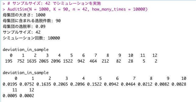
table(deviation_in_sample) |> print()
cat("\n")
# シミュレーションで得られた標本の逸脱件数の相対度数
(table(deviation_in_sample)/how_many_times) |> print()
cat("\n")# ヒストグラムの表示[標本の逸脱件数の度数]
hist_main = paste("Histogram of # of deviation in sample","\n","N=",N,"K=",K,"n=",n)
hist(deviation_in_sample, right = FALSE, main = hist_main, );box();}
# サンプルサイズ: 42 でシミュレーションを実施
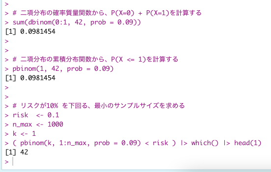
AuditSim(N = 1000, K = 90, n = 42, how_many_times = 10000)# 二項分布の確率質量関数から、P(X=0) + P(X=1)を計算する
sum(dbinom(0:1, 42, prob = 0.09))
# 二項分布の累積分布関数から、P(X <= 1)を計算する
pbinom(1, 42, prob = 0.09)
# リスクが10% を下回る、最小のサンプルサイズを求める
risk <- 0.1
n_max <- 1000
k <- 1
( pbinom(k, 1:n_max, prob = 0.09) < risk ) |> which() |> head(1)
実行例

資料集
清水公認会計士事務所 essays in some subjects: 統計
https://jicpa.or.jp/specialized_field/publication/files/2-24-530-2-20111114.pdf
2010 Attribute Sampling Plans
内部統制テスト・上限逸脱率の計算方法: Honeywar日記
https://www.saaj.or.jp/members/kaiho/201110SAAJKaihoNr128.pdf
内部統制は100回中8回間違えて良い - 内部統制ブログ(フジタヒロキ)
https://www.aicpa.org/publications/accountingauditing/keytopics/downloadabledocuments/sampling_guide_technical_notes.pdf
Workflow: Classical audit sampling • jfa
https://onlinelibrary.wiley.com/doi/pdf/10.1002/9781119448617.app1
「システム監査基準」及び「システム管理基準」の改訂について(METI/経済産業省)
https://www.ifac.org/system/files/downloads/translation_db_file_09.pdf
ガンマ関数とガンマ分布についてのポエム
統計学実践ワークブック第15章にて、"指数分布(λ)はガンマ分布(1, 1/λ)である"、というワンフレーズでつまずいたので、
復習を兼ねてポエムです。なお、以下の議論において、厳密性は度外視している。
ガンマ関数
定義
s > 0 とする。ガンマ関数Γ(s) は次式で定義される。
性質1: Γ(1) = 1
Γ(1) = 1である。
性質2: Γ(s) = (s-1)Γ(s-1)
Γ(s) = (s-1)Γ(s-1)である。
性質3: Γ(n) = (n-1)! where n ∈ ℕ
のとき、Γ(n) = (n-1)!である。
∵ 性質1と2より、ガンマ関数は
ガンマ分布
定義
a>0, b>0, x ∈(0,∞) として、確率密度関数f(x)が
と表される連続型確率分布を、ガンマ分布G(a, b) という。
モーメント母関数
X ~ G(a,b) としてモーメント母関数 を求める。
ここで とすると、
となる。
再生性
X ~ G(a1, b) , Y ~ G(a2, b) でXとYは互いに独立であるとする、この時 X+Yの分布はモーメント母関数を用いて
と表される。これは X+Y ~ G(a1+a2, b) に等しい。よってガンマ分布は再生性を持つ。
指数分布(λ)はガンマ分布(1, 1/λ)である
指数分布は確率密度関数が と表される。従って、ガンマ分布 G(a,b)にて
として求めると、
となり、確かに一致する。
マルコフ連鎖
統計学実践ワークブック問14.2より。
問題の概要
- 状態空間S = {1,2,3}
- マルコフ連鎖 X = (Xn)を以下に定める
- Xが状態iにあるとき、カードを1枚ランダムに引く。取り出したカードが
- a_i であれば状態iにとどまる
- a_j であれば
- 確率c_ij = min( j/i, 1 ) で状態jに推移
- 確率 1 - c_ij で iにとどまる
- Xが状態iにあるとき、カードを1枚ランダムに引く。取り出したカードが
- カードは復元抽出とする
- (1)マルコフ連鎖Xの確率推移行列Q を求めよ
問題の理解
どのカードもどーよーにたしからしく引く、つまり1/3の確率で引くことができると考える。 また、各状態で「とどまる」とはつまり、状態iから状態iに推移すると言い換えることができる。
これらの点に注意しながら、以下「状態2」について詳細に計算過程を記述する。 なお、カードは[1][2][3]で表し、状態は①②③で表すとする。また、分数および1と0は確率のことを指している。
- ②のとき
- 1/3で[1]を引き当てる
- 1/2で①へ推移 ⇔ 確率1/6で ②→①と状態推移する
- 1/2で[2]へ推移 ⇔ 確率1/6で ②→②と状態推移する
- 1/3で[2]を引き当てる
- 1で②へ推移 ⇔ 確率1/3で②→②と状態推移する
- 1/3で[3]を引き当てる
- 1で③へ推移 ⇔ 確率1/3で②→③と状態推移する
- 0で②へ推移 ⇔ 確率0で②→②と状態推移する
- 1/3で[1]を引き当てる
これを状態推移ごとにまとめると、
| 状態推移 | 確率 |
|---|---|
| ②→① | 1/6 |
| ②→② | 1/6 |
| ②→② | 1/3 |
| ②→③ | 1/3 |
| ②→② | 0 |
となって、図で表現すると


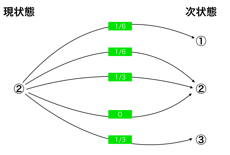

となる。
従って、確率推移行列の第2行の成分は(1/6,1/2,1/3)となる。
同様に考えると、
- 第1行の成分は(1/3,1/3,1/3)
- 第3行の成分は(1/9,2/9,2/3)
となる。
切断正規分布
統計学実践ワークブックの問6.1〔4〕は、いわゆる切断正規分布の問題である。このキーワードでググると良い。
なお、期待値を求めるために確率変数 のモーメント母関数を計算しようとすると怪我をする?ので、素直に
から定義通り期待値を求めましょう。
2022-02-19 追記
ワークブックに従い、素直に確率密度関数f(z) = (1/2)×ϕ(z) where z > 0 , 0 where z ≦ 0 と考えた方が楽。